Any-Precision Deep Neural Networks
2022.11.21
Deep dive into quantization Keywords: #Quantization
0. Abstract
- github code: https://github.com/SHI-Labs/Any-Precision-DNNs
- Proposal: Any-precision deep neural networks which are trained with a new method that allows the learned DNNs to be flexible in numerical precision during inference
- How? By truncating the least significant bits.
- Problem: Previous literature presents solutions to train models at fixed precision/accuracy trade-off point. $\rightarrow$ But how to produce a model flexible in runtime precision is largely unexplored
1. Introduction
- Previous literature
- Mixed-precision models: models with some layers processing in ultra-low precision and some layers in high precision
- Main Problem
- efficiency/accuracy trade-off always exists, so we have to find the right trade-off point, but what if we demand flexibility?
- That is, it would be favorable if we can dynamically change the efficiency/accuracy trad-off point given diffenert situations, without re-training or re-calibration
- Contributions
- In runtime, we can quantize its layers into various precision layers without fine-tuning or calibration and without any data . Accuracy changes smoothly w.r.t. its precision level without drastic performance degradation
- Any-precision DNN trains better low-bit models with KD
2. Related Work
- Low-Precision Deep Neural Networks
- Binarized Neural Networks, XNOR-Net
- Quantization Operator
- Straight Through Estimator(STE)
3. Any-Precision Deep Neural Networks
3.1 Overview
- N-bit fixed-point integers to represent weights($w_Q$) and input activations($x_Q$)
- Adding a layer-wise scaling factor $s$ helps reduce the output range variation and hence achieve better model accuracy.
- The activations $y’$ are then quantized into N-bit fixed-point integers
3.2 Inference
- Once training is finished, we can keep the weights at a higher precision level for storage e.g. 8 bits
- We quantize the weights into lower bit-width by bit-shifting (truncate)
3.3 Training
3.3.1 Quantization-aware training (QAT)
“Train the model taking quantization into consideration”
- A full precision copy of the weights W is maintained throught the training.
- Small gradients are accumulated without loss of precision → gradients effect the ‘full precision copy of weights’
- Once the model is trained, only the quantized weights are used for inference.
- BN layer is important in low-precision DNN
- $y’$ is first passed into the BN layer and THEN quantized into $y_Q$
3.3.2 Weights
- Uniform quantization strategy:
- Normalize weights to [0,1]:
graph
Where $\tanh(w)$ limits the range of weights to [-1,1] (normalize before quantization), and $\max|\tanh(w)|$ is the maximum taken over all weights in the layer. By construction, $\tanh(w)/\max|\tanh(w)|$ is still in the range of [-1,1]. Add 1 and half the value to keep the weights in a nice [0,1] range in order to proceed with the scaling step. (▲)
- Quantize normalized value into N-bit integer
Where $\text{MAX}_N$ denotes the upper-bound of N-bit integer. Because $w’$ is in range [0,1], we only need to multiply $\text{MAX}_N$ and round it to an integer to get $w_Q’$.
- Values remapped to approximate the range of floating point values to obtain
Do the reverse op. of (▲) so that $w_Q$ becomes the intended quantization. The rationale of multiplying expectation of the weights comes from XNOR-Net.
- Approximate $w$ with $s*w_Q$ Keeping track of how $w$ was scaled throughout the quantization process,multiply $s$ to the final quantized weight.
- Normalize weights to [0,1]:
- Forward Pass
- Execute feed-forward pass with quantized weights:
Overload of notation $s$ - (1) quantization scaling factor for weights, (2) layer-wise scaling factor to reduce output range variation
- Backward Pass
- Gradients are computed w.r.t the underlying float-value variable $w$(because we use the quantized version $w_Q$, in the feed-forward pass) and updates are applied to $w$ as well.
- Straight through estimator (STE): Used to approximate gradients
(ex) round op. has zero derivatives everywhere (why? because it’s a step function). With STE, the gradient of round op. is 1.
3.3.3 Activations
- Clipping: Clip acitvation values to be within [0,1]
3.3.4 Dynamic Model-wise Quantization
- Previous works: Bit-width N is fixed during the training process → In runtime if we alter N, accuracy drops drastically
- Proposal: Dynamically change N within the training stage to align the training and inference process
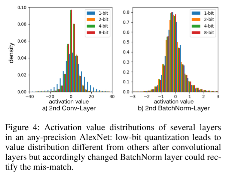
- Problem 1: Distribution of activations varies under different bit-width N, especially when N is small, failing to converge
- Solution 1: Adopt BN layer that calculates running average
- Problem 2: Still fails
- Solution 2: (Proposal) Adopt dynamically changed BN layer to work with different N in training. Parameters of all BatchNorm layers are kept after training and used in inference. Storage for each bitwidth BN layer is negligible.
3.3.5 Etc.
- Knowledge distillation: KD gives ~$\pm$1% boost
4. Experiments
4.1 Implementation Details
- For all models, first and last layer is real-valued.
- In training, we train the networks with bit-width candidates {1,2,4,8,32}
4.2 Comparison to Dedicated Models
- The proposed any-precision DNN generally achieved comparable performance to the competitive dedicated models.
- Any-precision model is more compact
4.3 Post-Training Quantization Methods
- Compared with three alternative post-training quantization method
- Directly quantizes dedicated models with bit-shifting (truncation)
- Simply drop LSB.
- Fails dramatically.
- Bit-shifting + BatchNorm calibration process
- Calibration process: BN statistics is recalculated by feed-forwarding a number of training samples
- Worked in 4-bit, but failed in 1, 2 bit settings
- ACIQ
- Analytical weight clipping, adaptive bit allocation, bias correction
- (Proposed Method) Calibrate the remaining 3, 5, 6, 7-bit settings to get the missed copies of BN layer params.
- In runtime we can freely choose any precision level from 1 to 8 bits.
- Directly quantizes dedicated models with bit-shifting (truncation)
4.4 Dynamically Change BN Layers
- Keeping multiple copies of BN layer params for different bit-widths → Minimized input variations to the convolutional layers → Allow same set of convolutional layer params. to support any-precision in run time
4.5 Ablation Studies
Candidate bit-width List
How does the candidate bit-width list used during training influence test performance on other bit-widths
- Training with more candidate bit-width generally leads to better generalization to the others.
- i.e. 1,2,4,8-bits combination is better than rest.
- Coverage of candidate bit-width matters.
- i.e. 1,8-bits combination performs more stable across different runtime bit-width compared with 2,8-bits, 4,8-bits combination