Learned Step Size Quantization
2024-01-09
Keywords: #Quantization
0. Abstract
- Proposal
- Builds upon existing methods for learning weights in quantized networks by improving how the quantizer itself is configured
- Introduce a novel means to estimate the task loss gradient at each weight and activation layer’s quantizer step size, such that it can be learned with other parameters.
1. Introduction
- Learned Step Size Quantization (LSQ): Use the training loss gradient to learn the step size parameter of a uniform quantizer for each weights/act layer.
- adsf
- asdf
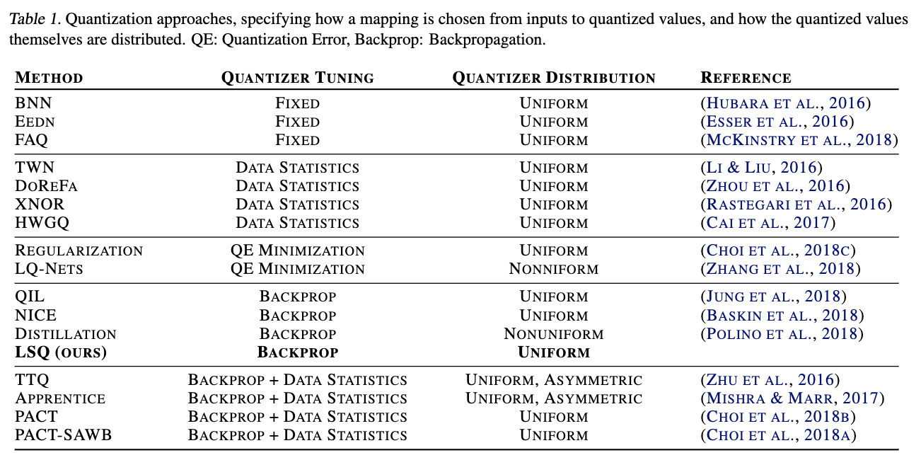
- Fixed mapping schemes: Simple, yet no guarantees on optimizing network performance.
- Quantization error minimization schemes: Optimal for minimizing quantization error, yet may be non-optimal if a different quantization mapping actually minimizes task error.
- LSQ vs Previous work using back-propagation:
- Usage of a different approximation to the quantizer gradient.
- Application of a scaling factor to the learning rate of the parameters controlling quantization.
2. Methods
2.0 Preliminaries
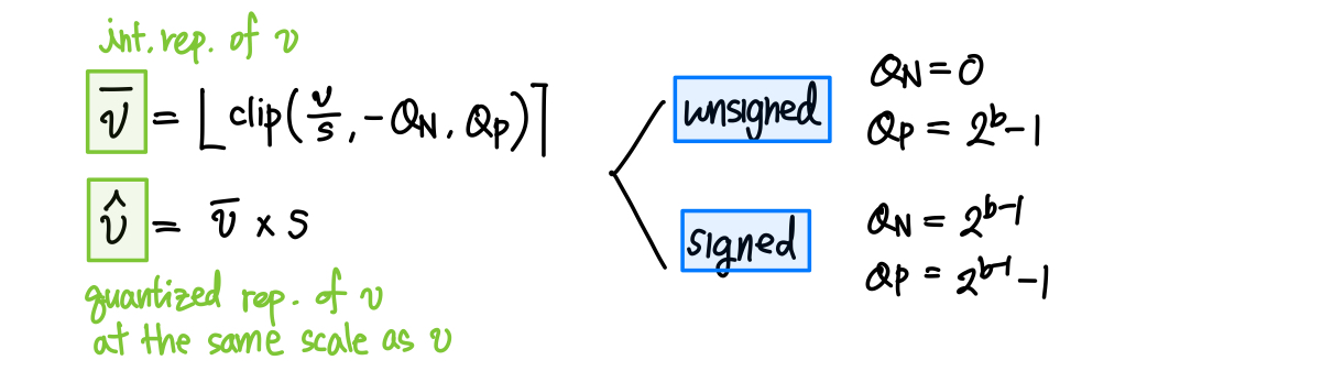
- For inference, we envision computing weights $w$ offline, for activations $x$ online, and using $\bar{w}, \bar{x}$ as input to low precision integer MM.
- Act. quant. function gradient: Use STE, and set the gradient of clipped values to zero.
- Weight quant. function gradient: Use STE, do not set gradient of clipped values to zero, as the weights can get permanently stuck in the clipped range.
2.1 Step Size Gradient
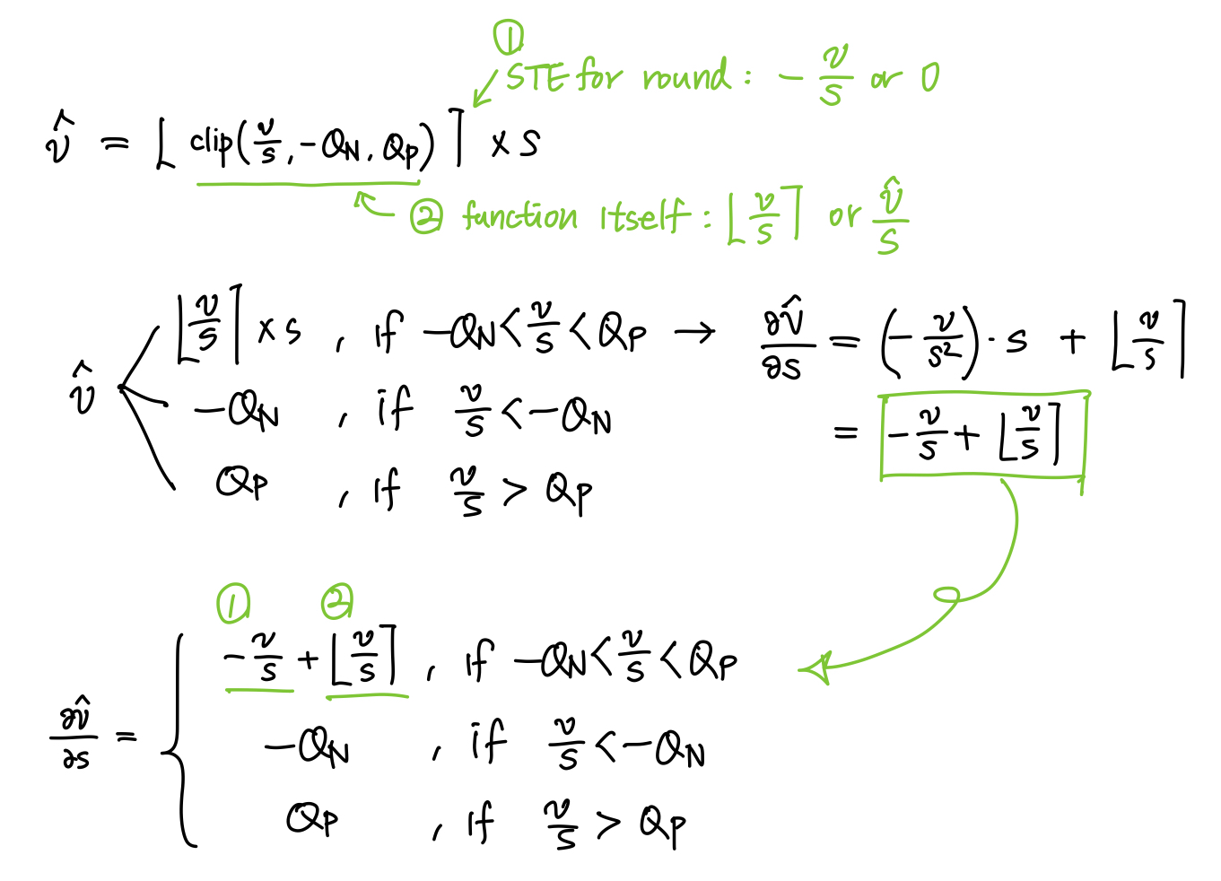
- Prior approaches: Completely remove the round operation when differentiating the forward pass.
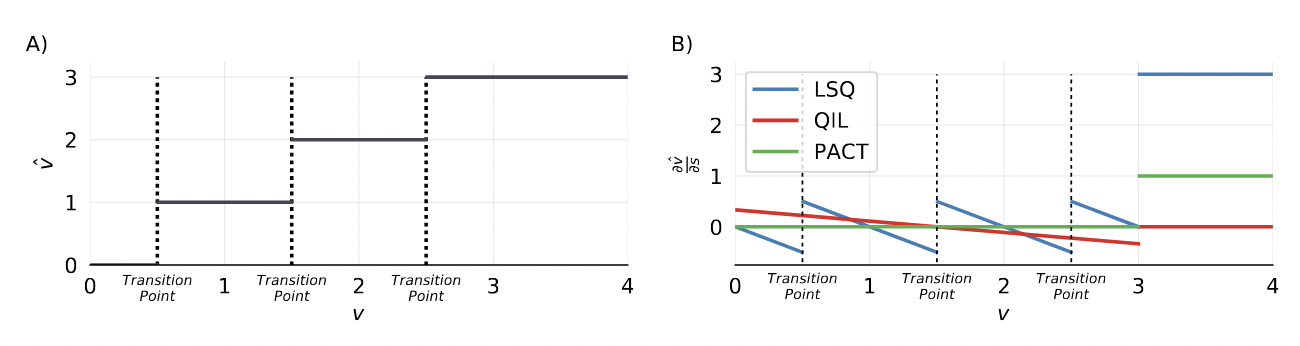
- For QIL and PACT, the relative proximity of $v$ to the transition point between quantized states does not impact the gradient to the quantization parameters.
- However, the closer a given $v$ is to a transition point, the more likely it is to change its quantization bin($\bar{v}$) as a result of a learned update to $s$ (since a smaller change in $s$ is required), thereby resulting in a large jump in $\hat{v}$
-
Thus, we would expect $\partial \hat{v}/\partial s$ to increase as the distance from $v$ to a transition point decreases.
- [# of step size params] = [# of quantized weight layers] + [# of quantized act. layers]
- Weight/Act. Initialization = $2<|v|>/\sqrt{Q_P}$
2.2 Step Size Gradient Scale
- (You et al., 2017) Ratio of update magnitude (lr) to parameter magnitude should be same for all weight layers for good convergence.
- Following this reasoning, step size (the learnable param. for LSQ), should also have its lr to param. magnitude proportioned similarly to that of weights.
- Thus, for a network trained on some loss $L$, the ratio below should be 1.
- $\nabla_s L / s$ : Ratio of lr to param. magnitude for step size
- $\lVert \nabla_w L \rVert / \lVert w \rVert$ : Ratio of lr to param. magnitude for weights
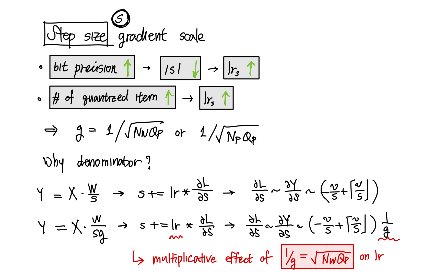
- Multiply step size loss by a grad_scale $g=1/\sqrt{N_WQ_P}$:
- Step size param. should be smaller as precision increases ← data is quantized more finely.
- Step size lr should be larger as the number of quantized items increases ← more items are summed across when computing its gradient.
2.3 Training
- Quantizers are trained with LSQ by making their step sizes learnable parameters with loss gradient computed using the quantizer gradient above.
- (Courbariaux et al., 2015) Training quantized networks: Full precision weights are stored and updated, quantized weights and activations are used for forward and backward passes, the gradient through the quantizer round function is computed using the STE (Bengoi et al., 2013) such that
-
Stochastic gradient descent
- We set input activations and weights to $\hat{a}$ and $\hat{w}$ except the first and last, which is always 8-bit → Making first and last layers high precision has become standard practice for quantized networks
- All other parameters are fp32
- All quantized networks are initialized using weights from a trained full precision model with equivalent architecture before fine-tuning in the quantized space (PTQ)
- Cosine learning rate decay without restarts (Loshchilov & Hutter, 2016)
- Under the assumption that the optimal solution for 8-bit networks is close to the full precision solution (McKinstry et al., 2018), 8-bit networks were trained for 1 epoch while all other networks were trained for 90 epochs.
3. Results
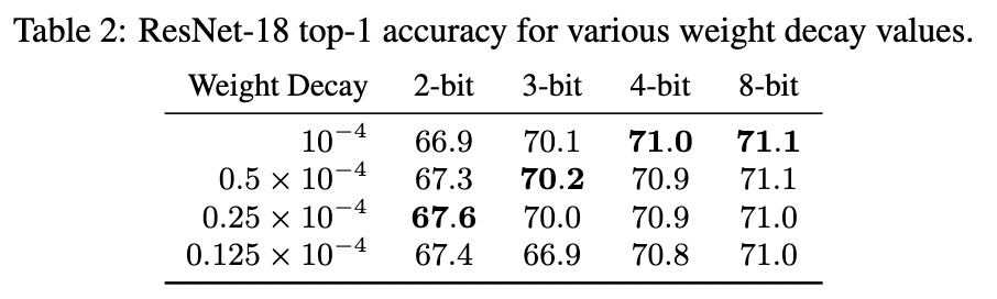
3.1 Weight Decay
- Reducing model precision reduces a model’s tendency to overfit, and thus reduce the need of regularization in the form of weight decay to achieve better performance
- Lower precision networks reach higher accuracy with less weight decay
3.2 Comparison with Other Approaches
- In some cases, we report slightly higher accuracy on full precision networks than in their original publications, which we attribute to our use of cosine learning rate decay (Loshchilov & Hutter, 2016).