Classification using Hyperdimensional Computing: A Review

2024-02-16

Keywords: #HDC

---

0. Abstract

• hypervectors: Unique data type for HD computing

1. Introduction

• HD computing represents different types of data using hypervectors, whose dimensionality is in the thousands (e.g. 10,000-$d$)
• Hypervectors are composed of IID components (binary, integer, real or complex)
• ✪ The concept of orthogonality

2. Background on HD Computing

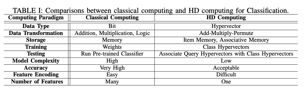
A. Classical Computing vs HD Computing

• Three key factors of computing: 1) Data representation, 2) data transformation, and 3) data retrieval
  • Data representation: Hypervector
  • Data transformation: Add-Multiply-Permute
  • Data retrieval: ?
• class hypervector: hvs generated from training data
• query hypervector: hvs generated from the test data

B. Data Representation

• Divided into two categories: binary or non-binary (bipolar, integer)
  • Non-binary hv: More hardware-friendly
  • Binary hv: Higher accuracy

C. Similarity Measurement

• Non-binary hv: cosine similarity
  • Only depend on orientation, focusing on the angle and ignoring the impact of magnitude.
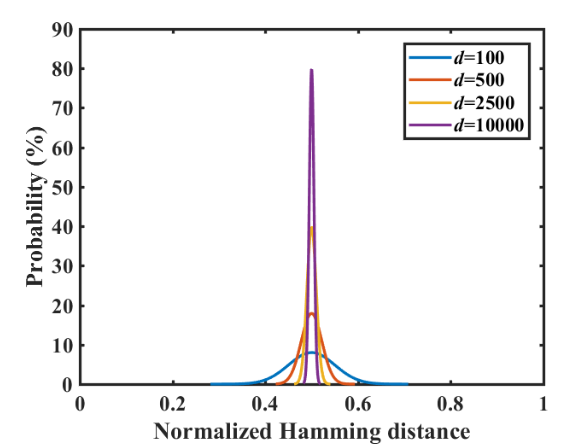
• Binary hv: normalized Hamming distance
• Orthogonality in high dimensions: Randomly generated hypervectors are nearly orthogonal to each other when $d$ is high.
• Orthogonal hvs = dissimilar: Operations performed on theses orthogonal hvs can form associations or relations.

D. Data Transformation

1. Bundling

• Pointwise addition
• Majority Rule

2. Binding

• Pointwise multiplication = XOR operation
• Aims to form associations between two related hypervectors
• $X = A \oplus B$ becomes otrthogonal to both $A$ and $B$

3. Permutation

• Circular right bit-shift
• $\text{Ham}(\rho (A), A) \sim 0.5$ for ultra-wide hvs

3. The HD Classification Methodology

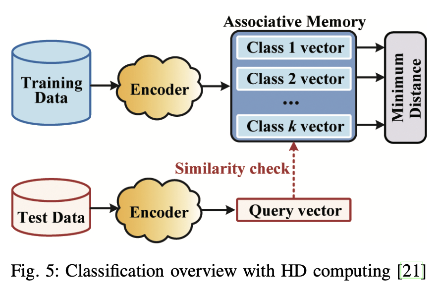
A. The HD Classification Methodology

1. The encoder employs randomly generated hvs to map training data to HD space.
2. A total of $k$ class hypervectors are trained and stored in the associative memory.
3. Inference phase: the encoder generates the query hv for each test data
4. Similarity check between the query hv and class hv in the associative memory.
5. The label with the closest distance is returned.

B. Encoding Methods for HD Computing

• Encoding: Mapping input data into hvs, somewhat similar to extraction of features
• Record-based Encoding
  • Position hvs: Randomly generated to encode the feature position information → Orthogonal to each other
  • Level hvs: The feature value information is quantized to $m$ level hvs. For an $N$-dim feature, a total of $N$ level hvs should be generated, which are chosen from the $m$ level hvs. → Randomly bit-flip $d/m$ ($d$ is dimension) to generate next level hv, the last-level hv being nearly orthogonal to the first hv.
  • Encoding: Bind each position hv with its level hv. The final encoding hv $\mathbf{H}$ is obtained by bundling.

• N-gram-based encoding
  • Random level hvs are generated, then feature values are obtained by permuting these level hvs.
  • (ex) the level hv $\bar{\mathbf{L}_i}$ corresponding to the $i$-th feature position is rotationally permuted by $(i-1)$ positions.
  • The final encoded hypervector $\mathbf{H}$ is obtained by binding each permuted level hvs.

• Kernel encoding ✪

C. Benchmarking Metrics in HD Computing

• Tradeoff between accuracy and efficiency.
• Accuracy: Appropriate choice of encoding method, and retraining iteratively (compared to single-pass training) improves the training accuracy.
• Efficiency
  • Algorithm: Dimension reduction
  • Hardware: Binarization (employing binary hvs instead of non-binary model), Quantization, Sparsity → HW acceleration anticipated combining HD computing with in-memory computing

---