Overcoming Oscillations in Quantization-Aware Training

2024-06-07

Keywords: #QAT #weightdistribution

0. Abstract

This paper delves into the phenomenon of weight oscillations and show that it can lead to a significant accuracy degradation due to wrongly estimated BN statistics.
We propose two novel QAT algorithms to overcome oscillations during training:
- Oscillation dampening
- Iterative weight freezing

1. Introduction

Main Problem: When using STE for QAT, weights seemingly randomly oscillate between adjacent quantization levels leading to detrimental noise during the optimization process.
Problem of weight oscillation: They corrupt the estimated inference statistics of the BN layer collected during training, leading to poor validation accuracy.
- Pronounced in low-bit quantization of efficient networks with depth-wise separable layers.
- Probable solution: BN statistics re-estimation
Our solution
- Oscillation dampening
- iterative freezing of oscillating weights

2. Oscillations in QAT

2.1. Quantization-aware training

Original weights: Will be referred to as latent weights or shadow weights
STE: We approximate the gradient of the rounding operator as 1 within the quantization limits.

$\frac{\partial \mathcal{L}}{\partial \mathbf{w}}=\frac{\partial \mathcal{L}}{\partial \widehat{\mathbf{w}}} \cdot \mathbf{1}_{n \leq \mathbf{w} / s \leq p}$

2.2. Oscillations

Side effect of STE: Implicit stochasticity during the optimization process → Due to latent weights oscillating around the decision boundary between adjacent quantized states.

What exactly does “implicit stochasticity” mean in this context? Inherent randomness that arises naturally from the system’s dynamics (oscillations during training) and not because of an explicitly introduced factor.
Toy regression example: Looks complicated, but really just the MSE between label and output of quantized model.

$\min _w \mathcal{L}(w)=\mathbb{E}_{\mathbf{x}}\left[\frac{1}{2}\left(\mathbf{x} w_*-\mathbf{x} q(w)\right)^2\right]$

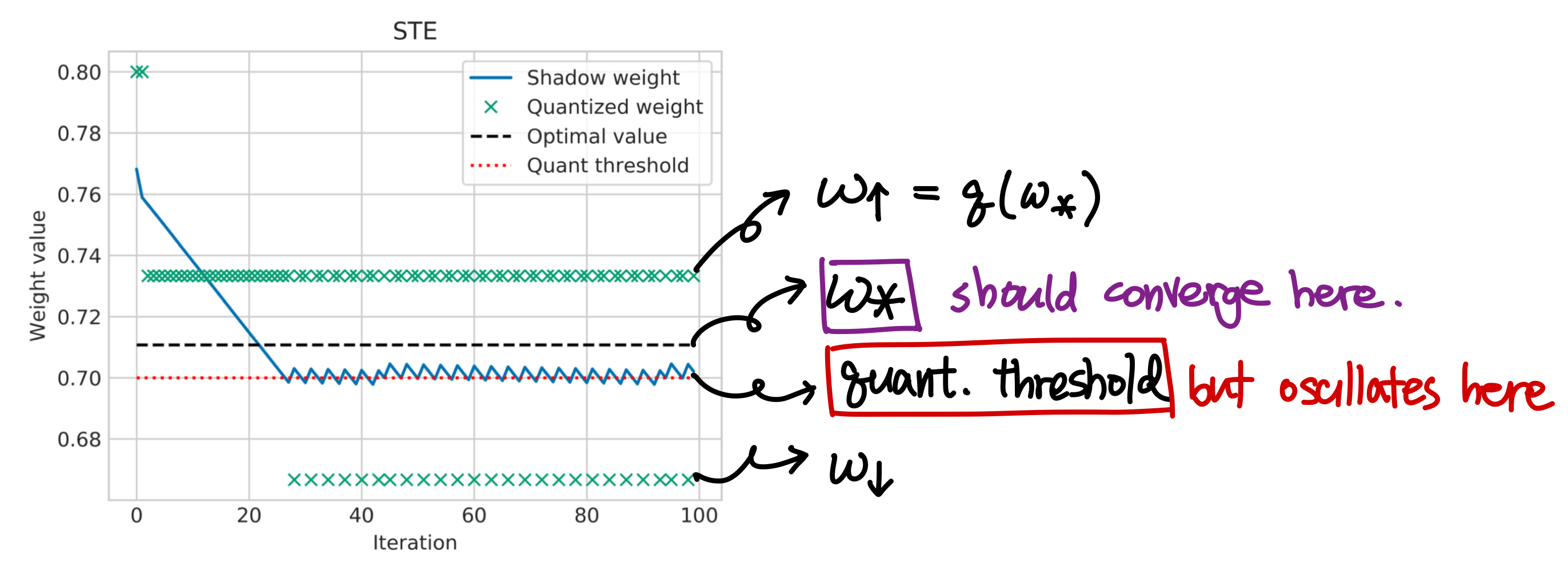
As the latent weight $w$ approaches the optimal value $w_\ast$, it starts oscillating around the decision threshold between- quantization level above the optimal value ($w_\uparrow$) and below ($w_\downarrow$)
Ideally, latent weight $w$ should converge to the optimal value ~~q(w_\ast)~~ $w_\ast$.

Why does this happen? When weights are above the threshold, STE pushes latent weight down towards $w_\downarrow$. When weights are below the threshold, STE push latent weight up towards $w_\uparrow$.
- When input is fixed, quantized weight will induce positive/negative gradients regardless of whether optimal weight is above/below the threshold. Therefore, weights oscillate near the threshold rather than the optimal value.
Frequency of oscillation: Dictated by the distance $d=|w_{\ast}-q(w_{\ast})|$
- Differentiate the equation from 2.Toy regression example.
- For more info, read Deep Dive: Overcoming Oscillations in QAT

2.3. Oscillations in practice

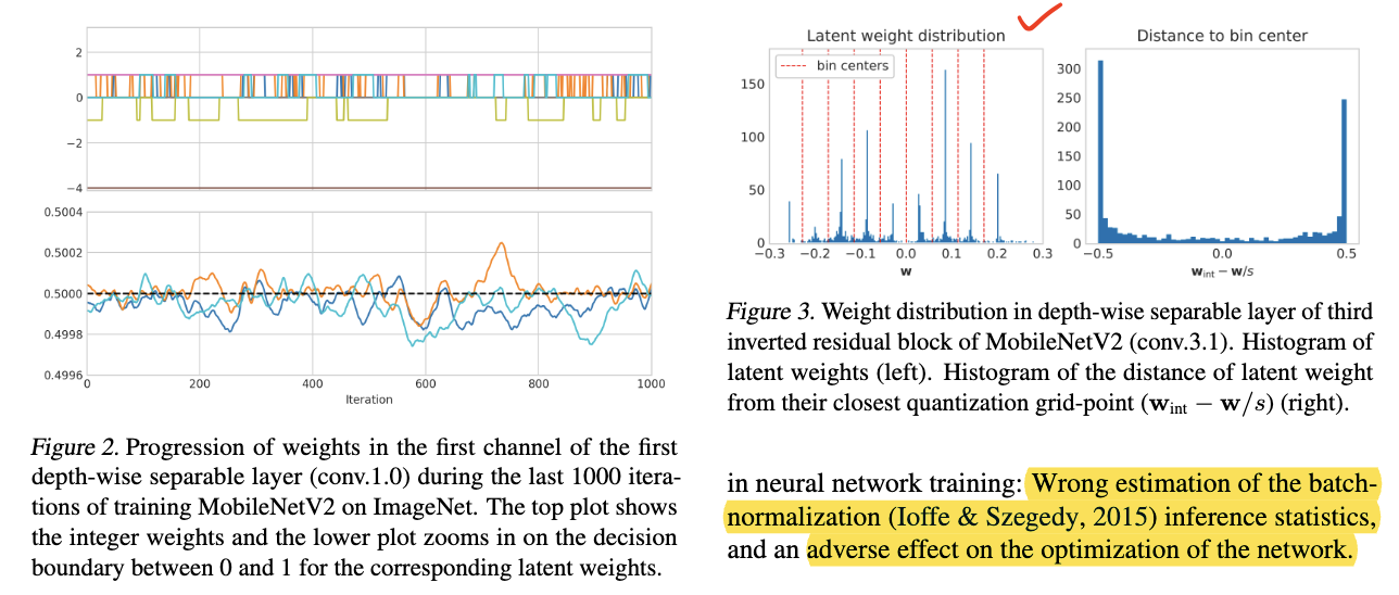
We observe that many of the weights appear to randomly oscillate between two adjacent quantization levels.
After the supposed convergence of the network, a large fraction of the latent weights lie right at the decision boundary between grid points.
- This reinforces the observation that a significant proportion of weights oscillate and cannot converge.

2.3.1. The effect on BN statistics

Output statistics of each layer vary significantly between gradient updates when weights oscillate.
Distribution shift by oscillations corrupt BN running estimates → Significant degradation in accuracy.
1. Bit-width $b$: Lower the bit-width, the distance between quantization levels becomes larger, as it is proportional to $1/2^b$. → Larger shift in output dist.
2. # of weights per output channel: Smaller the number of weights, the larger the contribution of individual weights to the final accumulation. When number is big enough, the effects of oscillations average out due to the law of large number.
  - Table 1 shows that KL divergence is much bigger for depth-wise separable layers (fewer weights) than point-wise convolutions (more weights).
  - Table 1 shows discrepancy between estimate and actual population statistics of BN following convolutional layers. → Discrepancy bewteen maximum and mean KL-divergence across the output channels of each layer.
Solution: Re-estimate the BN statistics with a small subset of data after training. → batch-normalization (BN) re-estimation
BN re-estimation not only 1) improves the final quantized accuracy, but also 2) reduces the variance among different seeds

2.3.2. The effect on training

??
Weight oscillations…
1. Prevent the network from converging to the best local minimum at the end of training.
2. Lead the optimizer towards sub-optimal directions earlier in training.

4. Overcoming oscillations in QATs

4.1. Quantifying Oscillations

Calculate frequency of oscillations over time using an exponential moving average (EMA)
For oscillation to occur, it needs to satisfy:
1. Integer value of the weight needs to change
2. Direction of change needs to be opposite than that of the previous change.
We then track the frequency of oscillations over time using EMA:

$f^t=m \cdot o^t+(1-m) \cdot f^{t-1}$

4.2. Oscillation dampening

When weights oscillate, they always move around the decision threshold between two quantization bins.
This means that oscillating weights are always close to the edge of the quantization bin.
In order to dampen the oscillatory behavior, we employ a regularization term that encourages latent weights to be close to the center of the bin rather than its edge.
Dampening loss (similar to weight decay):

$\mathcal{L}_{\text {dampen }}=\left\|s \cdot \mathbf{w}_{\text {int }}-\operatorname{clip}(\mathbf{w}, s n, s p)\right\|_F^2$

Final training objective is: $\mathbb{L}=\mathbb{L}\text{task}+\lambda\mathbb{L}\text{dampen}$

4.3. Iterative freezing of oscillating weights

Process
1. Track the oscillations frequency per weight during training.
2. If the oscillation frequency exceeds a threshold $f_{\text{th}}$, that weight gets frozen until the end of training.
When a weight oscillates, it does not necessarily spen an equal amount of time at both oscillating states.
To freeze the weight to its more frequent state, and therefor hopefully the state closer to the optimal value:
1. Keep a record of the previous integer values using an exponential moving average (EMA).
2. Assign the most frequent integer state to the frozen weight by rounding the EMA.

5. Experiments

5.1. Experimental Setup

Quantization
- LSQ for weight & activation quantization. Learn the quantization scaling factor.
- Keep weights of the first and last layer to 8-bits.
- Per-tensor quantization.
Optimization:
- In all cases; start from a pre-trained full-precision network. → This changes a lot of things.
- Instantial weight/activation quant. params. using MSE range estimation.
- SGD w/ $\text{momentum}=0.9$, cosine annealing learning-rate decay.

5.2. Ablation Studies

Oscillation Dampening
Iterative weight freezing
- Using a constant threshold: Smaller thresholds show lower percetage of oscillating weights at the end of training.
- Due to little osc. at the end of training, pre-BN re-estimation accuracy is closer to the post-BN.
  
  This means that, pre-BN acc. ↔ post-BN acc. can be an indication for whether oscillations remain at the end of training. Big difference $\propto$ large percentage of oscillating weights.

Problem: When threshold is too low, too many weights get frozen in the early stage of training. → Negatively affects the final accuracy.
Solution: Annealing schedule to the freezing threshold. → Allows a stronger freezing threshold and freeze almost all oscillations towards the end of training, when they are most disruptive.

Why are oscillations most disruptive at the end of training?

5.3. Comparison to other QAT Methods

Oscillation dampening method leads to an increase of about 33.3%
Iterative weight freezing has negligible computational overhead while achieving similar performance.