CSQ: Growing Mixed-Precision QuantizationScheme with Bi-level Continuous Sparsification

2024-07-26

---

1. Introduction

• Not all layers in a DNN are equally sensitive to quantization → Mixed-precision quantization
  • Sensitive layers keep higher precision, while less sensitive layers are quantized to lower precision.
• Main difficulty of mpq: Determining the exact precision of each layer.
  • RL-based search: Search-based method is costly to run.
  • Higher-order sensitivity stats. computed on the pretrained model: Pretrained model stats. do not capture the potential sensitivity changes during training.
  • Dynamically achieving mpq scheme through bit-level structural sparsity: 1) bit-level training process, 2) periodic precision adjustment → unstable convergence.
• Main contributions
  • Improve stability of bit-level training and adjustment to achieve better convergence.
  • Two main factors of instability:
    1. The binary selection of bit value.
    2. The binary selection of using a certain bit or ot in determining the precision of each layer.
  • Proposal: Continuous Sparsification Quantization (CSQ)
    • Continuous sparsification to relax discrete selection with a series of smooth parameterized gate functions.
    • Smoothness enables 1) fully differentiable training w/o gradient approximation (e.g. STE), 2) proper scheduling of the gate function parameter enables the model to converge w/o additional rounding.
    • +) consideration of budget constraints.
• Summary of contributions
  1. Utilize continuous sparsification technique to improve bit-level training of quantized DNN.
  2. Relax precision adjustment in the search of mpq scheme into smooth gate functions.
  3. Combine the bi-level continuous sparsification into effectively inducing high-performance mixed-precision DNNs.

2. Related Work

A. Mixed-precision quantization

• HAQ: Employs RL to determine quantization scheme -> Search costs can be high
• HAWQ: Measures each layer’s sensitivity with metrics like Hessian eigenvalue or Hessian trace.
  • Only incorporate the sensitivity of the pretrained full-precision model
  • Does not consider the change of sensitivity when weights are quantize/updated during QAT
• BSQ
  • Inaccurate STE gradient estimation.
  • Hard precision adjustment hinders convergence stability.
  • Solution: CSQ relaxes both bit-level training and precision adjustment with continuous sparsification

B. Sparse optimization and continuous sparsification

• Pruning: Binary mask used for selecting (or not selecting) a weight element/filter.
  • Minimizing $L_0$ regularization (= sum of the binary weight selection mask) induces sparsity.
  • Binary mask has a discrete nature. -> Attempts have been made to relax the binary constraint on the mask to enable gradient-based training.
• Continuous Sparsification (Smooth gating function)
  • Make closer approximations to the binary gate as training progresses.
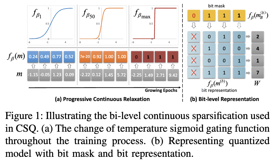
  • Relax the binary gate as a Sigmoid w/ temperature
  
  • Temp. $\beta$ controls the smoothness of the relaxed gate. Smaller $\beta$ for smoother optimization, larger $\beta$ to better approximate the discrete binary gate. $\beta$ grows as training progresses.

3. Method

A. Bi-level continuous sparsification of quantized DNN model

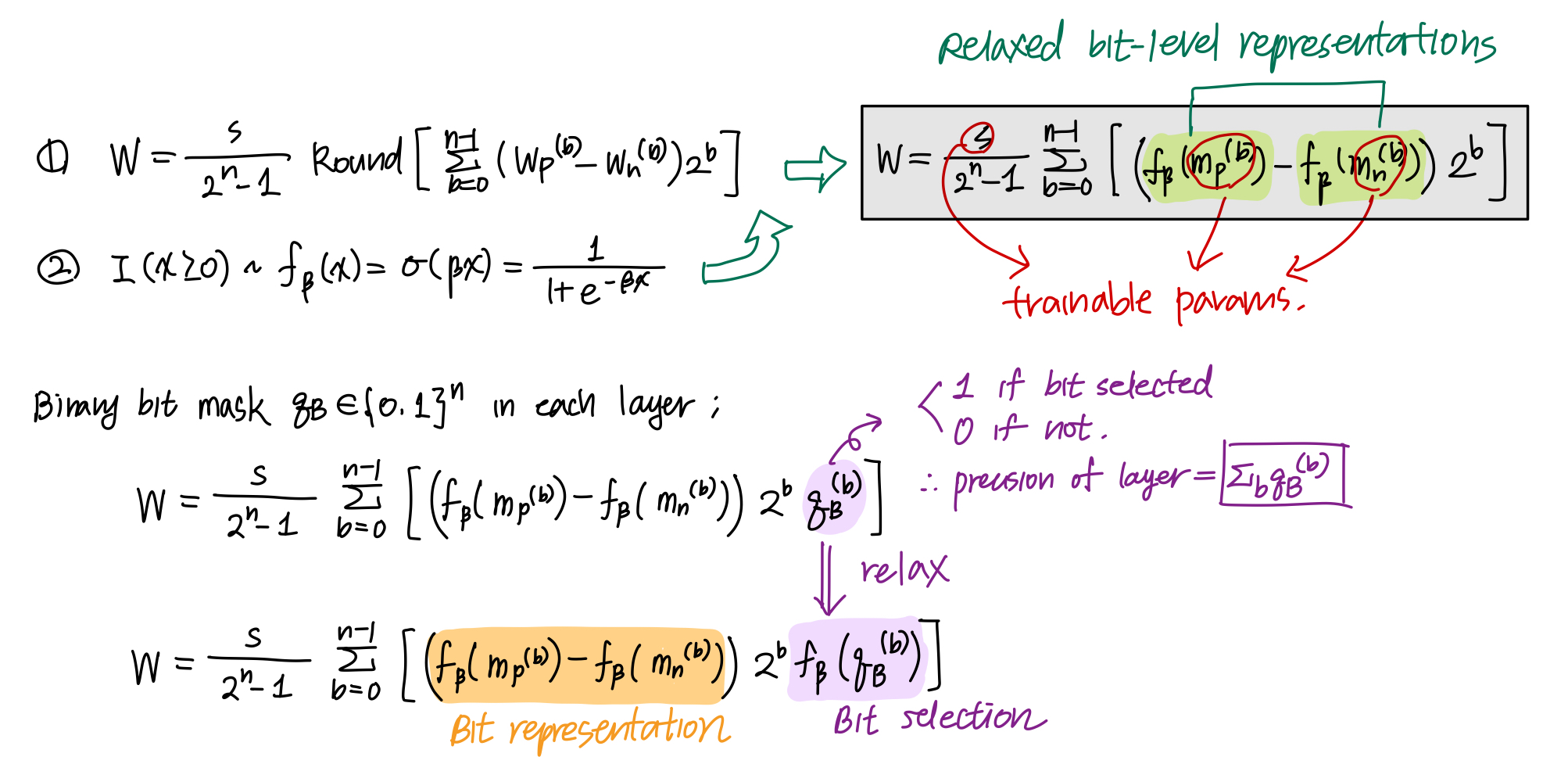
• To get a quantized model, we need: 1) The quantization precision of each layer 2) The quantized value of each weight element (w.r.t. each bit precision)
• Both are discrete properties, which prevent gradient-based updates.

• Discrete optimization -> Continuous differentiable function, to enable differentiable optimization.

• Continuous Sparsification
  • Exponentially increase $\beta$ with the # of epochs. Trainable params. can be optimized smoothly in the early training stage.
  • No rounding is applied -> No need for approximation of gradients.

B. Budget-aware growing of mixed-precision quantization scheme

• Adjust the precision of each layer using $l1$ regularization over the bit-mask of each layer $f_{\beta}(m_B^{(b)})$.
• Remember: $l1$ regularization induced sparsity.

• The final training objective:

• $\Delta_S$: Budget-aware scaling factor
  • More pruning when model size is bigger than the budget, and vice versa.
  • $\Delta_S = \text{Avg. precision of the model} - \text{Target avg. precision of the budget}$
• Precision is determined as $\sum_b [m_B^{(b)} \geq 0]$
• Training objective is end-to-end differentiable w.r.t. all learnable params, w/o using STE.

C. Overall training algorithm

• Sigmoid temp. $\beta$ is scheduled to grow exponentially with training epochs, where $f_{\beta}$ converges to a unit step Sign function.
• For ImageNet: Additional finetuning needed.
  • Fix the quantization scheme of each layer.
  • Only finetune the bit representation $s, m_p, m_n$ of the selected bits in each layer.
  • Rewind temp $\beta$ back to 1 and redo exponential temp. scheduling. (for bit representation only)

4. Evaluation

A. Experimental Setup.

---