BSQ: Exploring Bit-Level Sparsity for Mixed Precision Neural Network Quantization

2024-08-23

---

1. Introduction

• Model compression aims 1) to reduce model size, 2) while maintaining performance. The two optimization objectives have a contrary nature:
  1. A differentiable loss function $\mathbb{L}(W)$ w.r.t. the model’s weights $W$
  2. Model size, measured by the # of non-zero params. or ops., is a discrete function.
• Previous works to co-optimize performance and model size: Relax the representation of model size as a differentiable regularization term $R(W)$.
  • $\mathbb{L}(W)+\alpha R(W)$: $\alpha$ governs the performance-size tradeoff.

• Problem: There lacks a well-defined differentiable regularization term that can effectively induce quantization schemes.

• Previous works on quantization.
  • Apply the same precision to the entire model → Still incurs significant accuracy loss, even after integrating emerging training techniques
  • Different layers of a model present different sensitivities with performance, hence mixed-precision quantization scheme is ideal for performance-size tradeoff.
  • Problem:
    1. Exhaustively explore the search space which grows exponentially with the # of layers.
    2. The dynamic change of each layer’s precision cannot be formulated into a differentiable objective.
  • NAS suffers from extremely high searching cost.
  • Rank each layer based on the corresponding Hessian information (Dong et al.) → Need to manually select precision level for each layer.
• Proposal: Revisit fixed-point quantization from a new angle; bit-level sparsity
  • Precision reduction = Increasing layer-wise bit-level sparsity.
  • Consider each bit of fixed-point params. as continuous trainable variables.
  • Utilize a sparsity-inducing regularizer to explore the bit-level sparsity with gradient-based optimization.
• Contribution
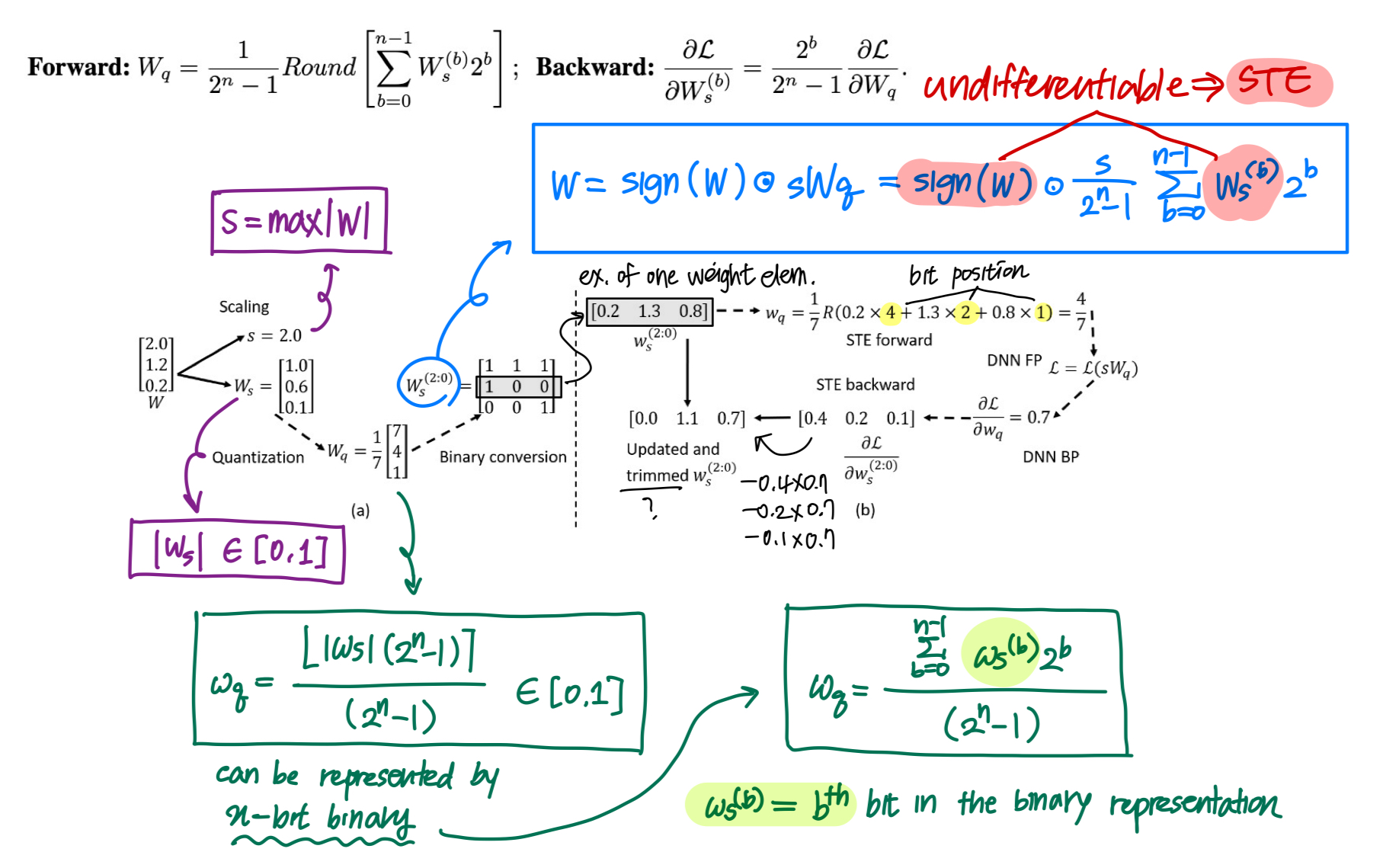
  1. Gradient-based training for bit-level quantized DNN models. Each bit of quantized weights is an independent trainable variable and enables gradient-based optimization with STE.
  2. Bit-level group Lasso regularizer to dynamically reduce the weight precision of every layer.
  3. bSQ uses only one hyperparameter- the strength of the regularizer, to trade-off the model performance and size, making the search more efficient.

3. The BSQ Method

3.1 Training the Bit Representation of DNN

• Memory overhead: $N$-bit model in bit representation will have $N$ times more parameters and gradients to be stored comparing to that of baseline.
  • Hidden feature (layer outputs) consumes a significantly larger memory than weights and gradients.
• Compute overhead: Gradient w.r.t. each $W_s^{(b)}$ can be computed as the gradient w.r.t. the corresponding $W_q$ scaled by a power of 2. Under $N$-bit scheme, there will only be $N$ additional scaling for each parameter comparing to baseline.
  • Very cheap compared to floating-point operations involved in backprop.

• Clamp $W_s^{(b)}$ within [0,2], so that $W_q$ has the chance to increase or decrease its precision in the “precision adjustment” step. (In Sec 3.3)

• Dynamic update of $sign(W)$ : Separate pos/neg elements in $W_s$
  • $W_s = (W_p-W_n)$ before quantization. → Separate pos/neg beforehand, so we only need to add (-) to the according weight elements.
  • $W_p = W_s \odot \mathbb{1}(W_s\geq 0)$ : All positive values
  • $W_p = W_s \odot \mathbb{1}(W_s < 0)$ : All absolute negative values
  • $W_s = (W_p-W_n)$ → $W_s^{(b)} = (W_p^{(b)}-W_n^{(b)})$

3.2 Bit-Level Group Lasso

• Why Lasso regularizer? To induce sparsity, which leads to precision reduction in the context of bit precision quantization.
• Bit-level group Lasso ($B_{GL}$) regularizer

• $[\cdot ; \cdot]$ : Denotes the concatenation of matrices.
• When, $B_{GL}$ could make a certain bit $b$ of all elements in both $W_p^{(b)}$ and $W_n^{(b)}$ zero simultaneously, the bit can be safely removed for precision reduction.

3.3 Overall Training Process

1. Convert each layer of FP model → 8-bit fixed-point
2. BSQ training with bit-level group Lasso integrated into the training objective
3. Re-quantization steps conducted periodically to identify bit-level sparsity induced by the regularizer → dynamic precision adjustment
4. The finalized mixed-precision quantization scheme is finetuned.

Objective of BSQ training

• Memory consumption-aware reweighing to $B_{GL}$ across layers. → Penalize layers with more bits.
• Layer-wise adjustment in the regularization strength by applying stronger regularization on a layer with higher memory usage.

Re-quantization and precision adjustment

• BSQ trains the bit representation of the model with floating-point values.
• Re-quantization: Convert $W_p^{(b)}$ and $W_n^{(b)}$ to binary values to identify the all-zero bits that can be removed for precision reduction.
• $W_p^{(b)}, W_n^{(b)} \in [0,2]$, the reconstructed $W_q’ = \lfloor\sum_{b=0}^{n-1}W_p^{(b)}2^b-\sum_{b=0}^{n-1}W_n^{(b)}2^b\rceil$

Activation quantization

• BSQ predetermines the activation precision and fix it throughout the BSQ training process.
• RELU-6 for layers $\geq$4-bit, PACT for layers <4-bit.

Post-training finetuning

• Final re-quantization and precision adjustment to get the final mixed-quantization scheme.
• Further finetuned using QAT.

---